Lesson 17 - Gradient and pattern

In this lesson, we'll explore how to implement gradients and repeating patterns.

• Use CanvasGradient to implement gradients
  • Imperative. Create textures using the Device API
  • Declarative. Supports CSS gradient syntax: linear-gradient, radial-gradient, conic-gradient
  • Use Shoelace to implement gradient configuration panel
• Use Shader to implement Mesh Gradient
  • Simulate random
  • Value Noise and Gradient Noise
  • Voronoi, FBM and Domain Warping
• Export SVG
• Use CanvasPattern to implement repeating patterns

Use CanvasGradient

We can use the CanvasGradient API to create various gradient effects, which can then be consumed as textures. We'll introduce both imperative and declarative implementations.

Creating Gradient Textures Imperatively

Taking linear gradient as an example, after creating a <canvas> and getting its context, createLinearGradient requires start and end points that define the gradient's direction. Then add multiple color stops, draw to the <canvas>, and use it as a source for creating textures:

const gradient = ctx.createLinearGradient(0, 0, 1, 0); // x1, y1, x2, y2

gradient.addColorStop(0, 'red');
gradient.addColorStop(1, 'blue');

ctx.fillStyle = gradient;
ctx.fillRect(0, 0, 256, 1);

Create a texture object using the Device API, and finally pass it to the shape's fill property to complete the drawing.

// 0. Create gradient data
const ramp = generateColorRamp({
    colors: [
        '#FF4818',
        '#F7B74A',
        '#FFF598',
        '#91EABC',
        '#2EA9A1',
        '#206C7C',
    ].reverse(),
    positions: [0, 0.2, 0.4, 0.6, 0.8, 1.0],
});

// 1. Get canvas device
const device = canvas.getDevice();

// 2. Create texture object
const texture = device.createTexture({
    format: Format.U8_RGBA_NORM,
    width: ramp.width,
    height: ramp.height,
    usage: TextureUsage.SAMPLED,
});
texture.setImageData([ramp.data]); // Pass the previously created <canvas> data to texture

// 3. Pass the texture object to the shape's `fill` property
rect.fill = { texture };

However, we want to support declarative syntax to improve usability and facilitate serialization.

Declarative CSS Gradient Syntax

Following CSS gradient syntax, we can use gradient-parser to obtain structured results, which can then be used to call APIs like createLinearGradient:

rect.fill = 'linear-gradient(0deg, blue, green 40%, red)';
rect.fill = 'radial-gradient(circle at center, red, blue, green 100%)';

The parsing results are as follows:

linearGradient = call(() => {
    const { parseGradient } = Core;
    return parseGradient('linear-gradient(0deg, blue, green 40%, red)');
});

radialGradient = call(() => {
    const { parseGradient } = Core;
    return parseGradient(
        'radial-gradient(circle at center, red, blue, green 100%)',
    );
});

There are several common gradient types, and we currently support the first three:

• linear-gradient Supported by CSS and Canvas
• radial-gradient Supported by CSS and Canvas
• conic-gradient Supported by CSS and Canvas
• repeating-linear-gradient Supported by CSS, can be hacked with Canvas, see How to make a repeating CanvasGradient
• repeating-radial-gradient Supported by CSS
• sweep-gradient Supported in CanvasKit / Skia

Additionally, we support overlaying multiple gradients, for example:

rect.fill = `linear-gradient(217deg, rgba(255,0,0,.8), rgba(255,0,0,0) 70.71%),
    linear-gradient(127deg, rgba(0,255,0,.8), rgba(0,255,0,0) 70.71%),
    linear-gradient(336deg, rgba(0,0,255,.8), rgba(0,0,255,0) 70.71%)`;

Gradient Editor Panel

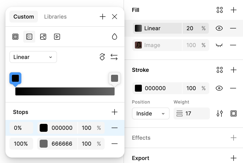
Inspired by Figma's gradient editing panel, we've implemented a similar editor. You can trigger the editing panel by selecting a shape in the example above.

Figma gradient panel

Implementing Gradients with Mesh

The gradients implemented based on Canvas and SVG have limited expressiveness and cannot display complex effects. Some design tools like Sketch / Figma have many Mesh-based implementations in their communities, such as:

• Mesh gradients plugin for Sketch
• Mesh Gradient plugin for Figma
• Photo gradient plugin for Figma
• Noise & Texture plugin for Figma

We referenced some open-source implementations, some implemented in Vertex Shader, others in Fragment Shader. We chose the latter:

• meshgradient
• Mesh gradient generator
• react-mesh-gradient

Due to WebGL1 GLSL100 syntax compatibility, we need to avoid using switch, otherwise we'll get errors like:

CAUTION

ERROR: 0:78: 'switch' : Illegal use of reserved word

Also, in for loops, we cannot use Uniform as the termination condition for index:

CAUTION

ERROR: 0:87: 'i' : Loop index cannot be compared with non-constant expression

Therefore, we can only use constant MAX_POINTS to limit loop iterations, similar to Three.js chunks handling light sources:

#define MAX_POINTS 10

for (int i = 0; i < MAX_POINTS; i++) {
    if (i < int(u_PointsNum)) {
        // ...
    }
}

Now let's dive into the details of Shaders. You can refer to The Book of Shaders - Generative Design to learn more details.

Random

To implement noise effects, we need a random function. However, GLSL does not have a built-in random function, so we need to simulate this behavior. Since it's a simulation, for the same random(x), we always get the same return value, so it's a pseudo-random number.

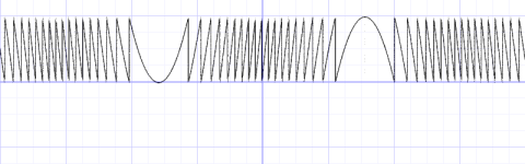
If we want to get a random function that returns a value between 0 and 1, we can use y = fract(sin(x)*1.0);, which only retains the decimal part.

y = fract(sin(x)*1.0)

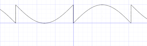
Observing this function, we can find that if we reduce the period to be extremely short, the values corresponding to the same x can be considered approximately random (pseudo-random). The specific method is to increase the coefficient, for example y = fract(sin(x)*10.0);.

y = fract(sin(x)*10.0)

Further increasing to 100000, we can no longer distinguish the waveform of sin. It's important to note again that unlike Math.random() in JS, this method is deterministic random, and its essence is actually a hash function.

We need to apply the random function to a 2D scene, where the input changes from a single x to an xy coordinate. We need to map the 2D vector to a single value. The book of shaders uses the dot built-in function to multiply a specific vector, but it doesn't explain why.

float random (vec2 st) {
    return fract(sin(
        dot(st.xy,vec2(12.9898,78.233)))*
        43758.5453123);
}

After searching online, we found this answer What's the origin of this GLSL rand() one-liner?。It's said that it originally came from a paper, and there's no explanation for why the three Magic Numbers are chosen. Anyway, the generated effect is good, similar to the "snow screen" of a black and white TV. You can see this effect by increasing the NoiseRatio in the example above.

Value noise

Using our defined random function, and floor, we can get a step-like function.

float i = floor(x);
y = random(i);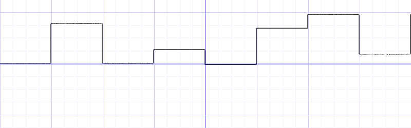

step

If we want to interpolate between adjacent "steps", we can use a linear function or a smooth interpolation function smoothstep:

float i = floor(x);
float f = fract(x);
y = mix(rand(i), rand(i + 1.0), f);
// y = mix(rand(i), rand(i + 1.0), smoothstep(0.,1.,f));

smoothstep

In one dimension, we chose i+1, and in two dimensions, we can choose the 4 adjacent points. The corresponding mixing function also needs to be modified. The mixing function in the original text is the expanded form, which is a bit difficult to understand, but the benefit is that it calls mix twice less.

float noise (in vec2 st) {
    vec2 i = floor(st);
    vec2 f = fract(st);

    // Four corners in 2D of a tile
    float a = random(i);
    float b = random(i + vec2(1.0, 0.0));
    float c = random(i + vec2(0.0, 1.0));
    float d = random(i + vec2(1.0, 1.0));

    vec2 u = smoothstep(0.,1.,f);

    // Mix 4 coorners percentages
    return mix(a, b, u.x) +
            (c - a)* u.y * (1.0 - u.x) +
            (d - b) * u.x * u.y;

    // It's actually the expanded form below
    return mix( mix( a, b , u.x),
                mix( c, d, u.x), u.y);
}

The above method of generating noise is interpolation between random values, so it's called "value noise". Carefully observing it, we can find that this method generates results with obvious blocky traces, such as the left part in the example below.

Gradient noise

In 1985, Ken Perlin developed another noise algorithm called Gradient Noise. Ken solved how to insert random gradients (gradients, gradients) instead of a fixed value. These gradient values come from a two-dimensional random function, which returns a direction (a vector in vec2 format) instead of a single value (float format).

The specific algorithm is as follows, and the biggest difference from value noise is the use of dot to interpolate the four directions:

float noise( in vec2 st ) {
    vec2 i = floor(st);
    vec2 f = fract(st);

 vec2 u = smoothstep(0., 1., f);

    return mix( mix( dot( random( i + vec2(0.0,0.0) ), f - vec2(0.0,0.0) ),
                     dot( random( i + vec2(1.0,0.0) ), f - vec2(1.0,0.0) ), u.x),
                mix( dot( random( i + vec2(0.0,1.0) ), f - vec2(0.0,1.0) ),
                     dot( random( i + vec2(1.0,1.0) ), f - vec2(1.0,1.0) ), u.x), u.y);
}

For Ken Perlin, the success of his algorithm was far from enough. He felt it could be better. At the Siggraph in 2001, he showed "simplex noise".

The specific implementation can be found in: 2d-snoise-clear, and there's also a 3D version.

Voronoi noise

We already learned how to divide space into small grid areas in the "Drawing Pattern" section. We can generate a random feature point for each grid, and for a fragment within a grid, we only need to calculate the minimum distance to the feature points in the 8 adjacent grids, which greatly reduces the amount of computation. This is the main idea of Steven Worley's paper.

The random feature points use the random method we learned earlier, since it's deterministic random, the feature points within each grid are fixed.

// Divide the grid
vec2 i_st = floor(st);
vec2 f_st = fract(st);
float m_dist = 1.;
// 8 directions
for (int y= -1; y <= 1; y++) {
    for (int x= -1; x <= 1; x++) {
        // Current adjacent grid
        vec2 neighbor = vec2(float(x),float(y));
        // Feature point in adjacent grid
        vec2 point = random2(i_st + neighbor);
        // Distance from fragment to feature point
        vec2 diff = neighbor + point - f_st;
        float dist = length(diff);
        // Save the minimum value
        m_dist = min(m_dist, dist);
    }
}
color += m_dist;

The voronoi noise implementation based on this idea can be found in lygia/generative.

fBM

See Inigo Quilez's fBM, the noise can be value noise or gradient noise:

So we are going to use some standard fBM (Fractional Brownian Motion) which is a simple sum of noise waves with increasing frequencies and decreasing amplitudes.

The original text also explains in detail the reason for using gain = 0.5, which corresponds to H = 1. H reflects the "self-similarity" of the curve, used in procedural generation to simulate natural shapes like clouds, mountains, and oceans:

$$G=2^{-H}$$

const int octaves = 6;
float lacunarity = 2.0;
float gain = 0.5;

float amplitude = 0.5;
float frequency = 1.;

for (int i = 0; i < octaves; i++) {
 y += amplitude * noise(frequency*x);
 frequency *= lacunarity;
 amplitude *= gain;
}

See Inigo Quilez's Domain Warping and Mike Bostock's Domain Warping. Call fbm recursively:

f(p) = fbm( p )
f(p) = fbm( p + fbm( p ) )
f(p) = fbm( p + fbm( p + fbm( p )) )

Exporting Gradients to SVG

Linear Gradient

SVG provides linearGradient and radialGradient, but their supported attributes are quite different from CanvasGradient.

Conic Gradient

Refer to SVG angular gradient for an approximate implementation. The CSS conic-gradient() polyfill approach is to render using Canvas and export as dataURL, then reference it with <image>.

Multiple Gradient Overlay

For multiple gradient overlays, in Canvas API, you can set fillStyle multiple times for overlaying. In declarative SVG, you can use multiple <feBlend> to achieve this.

Implementing Patterns

We can use Canvas API's createPattern to create patterns, supporting the following syntax:

export interface Pattern {
    image: string | CanvasImageSource;
    repetition?: 'repeat' | 'repeat-x' | 'repeat-y' | 'no-repeat';
    transform?: string;
}

rect.fill = {
    image,
    repetition: 'repeat',
};

The string-based transform needs to be parsed into mat3, and then passed to setTransform.